TABLE 15-9
Many factors determine the attendance at Major League Baseball games. These factors can include when the game is played, the weather, the opponent, whether or not the team is having a good season, and whether or not a marketing promotion is held. Data from 80 games of the Kansas City Royals for the following variables are collected.
ATTENDANCE = Paid attendance for the game
TEMP = High temperature for the day
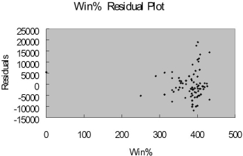
WIN% = Team's winning percentage at the time of the game
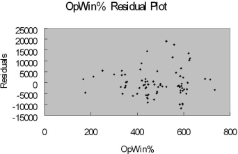
OPWIN% = Opponent team's winning percentage at the time of the game WEEKEND - 1 if game played on Friday, Saturday or Sunday; 0 otherwise PROMOTION - 1 = if a promotion was held; 0 = if no promotion was held
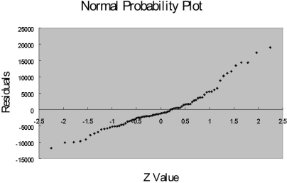
The regression results using attendance as the dependent variable and the remaining five variables as the independent variables are presented below.
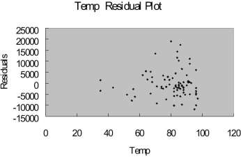
-Referring to Table 15-9, what is the correct interpretation for the estimated coefficient for TEMP?
Definitions:
Nonalcoholic Fatty Liver Disease (NAFLD)
A range of liver conditions affecting people who drink little to no alcohol, characterized by excessive fat stored in liver cells.
Hepatic Angiomatosis
A rare vascular disorder involving an increase in the number of blood vessels in the liver, leading to the formation of benign liver lesions.
Hepatic Sclerosis
A condition involving the hardening or scarring of the liver tissue, affecting liver function.
Chronic Lobular Hepatitis
A long-term inflammation of the liver affecting the lobules, potentially leading to liver damage.
Q14: Referring to Table 13-2, what is the
Q22: Referring to Table 18-3, suppose the
Q25: Referring to Table 15-4, given a quadratic
Q27: The Paasche price index is a form
Q57: The Shewhart-Deming cycle plays an important role
Q62: Referring to Table 14-3, to test whether
Q70: Referring to Table 17-1, what is the
Q116: Blossom's Flowers purchases roses for sale for
Q131: Referring to Table 14-16, the alternative hypothesis
Q192: Referring to Table 13-3, the standard error