TABLE 15- 8
the Superintendent of a School District Wanted

question 81

Multiple Choice

TABLE 15- 8
The superintendent of a school district wanted to predict the percentage of students passing a sixth- grade proficiency test. She obtained the data on percentage of students passing the proficiency test (% Passing) , daily average of the percentage of students attending class (% Attendance) , average teacher salary in dollars (Salaries) , and instructional spending per pupil in dollars (Spending) of 47 schools in the state.
Let Y = % Passing as the dependent variable, X₁ = % Attendance, X₂ = Salaries and X₃ = Spending.
The coefficient of multiple determination (R ² _j) of each of the 3 predictors with all the other remaining predictors are,respectively, 0.0338, 0.4669, and 0.4743.
The output from the best- subset regressions is given below:

$\begin{array}{llcclcc} & & & && \text {Adjusted} \\\text {Model }&\text { Variables} & \mathrm{Cp} & \mathrm{k} &\text {R Square} & \text {R Square} & \text {Std. Error }\\\hline 1 & X1 & 3.05 & 2 & 0.6024 & 0.5936 & 10.5787 \\2 & X1X2 & 3.66 & 3 & 0.6145 & 0.5970 & 10.5350 \\3 & X1X2X3 & 4.00 & 4 & 0.6288 & 0.6029 & 10.4570 \\4 & X1X3 & 2.00 & 3 & 0.6288 & 0.6119 & 10.3375 \\5 & X2 & 67.35 & 2 & 0.0474 & 0.0262 & 16.3755 \\6 & X2X3 & 64.30 & 3 & 0.0910 & 0.0497 & 16.1768 \\7 & X3 & 62.33 & 2 & 0.0907 & 0.0705 & 15.9984 \\\hline\end{array}$

Following is the residual plot for % Attendance: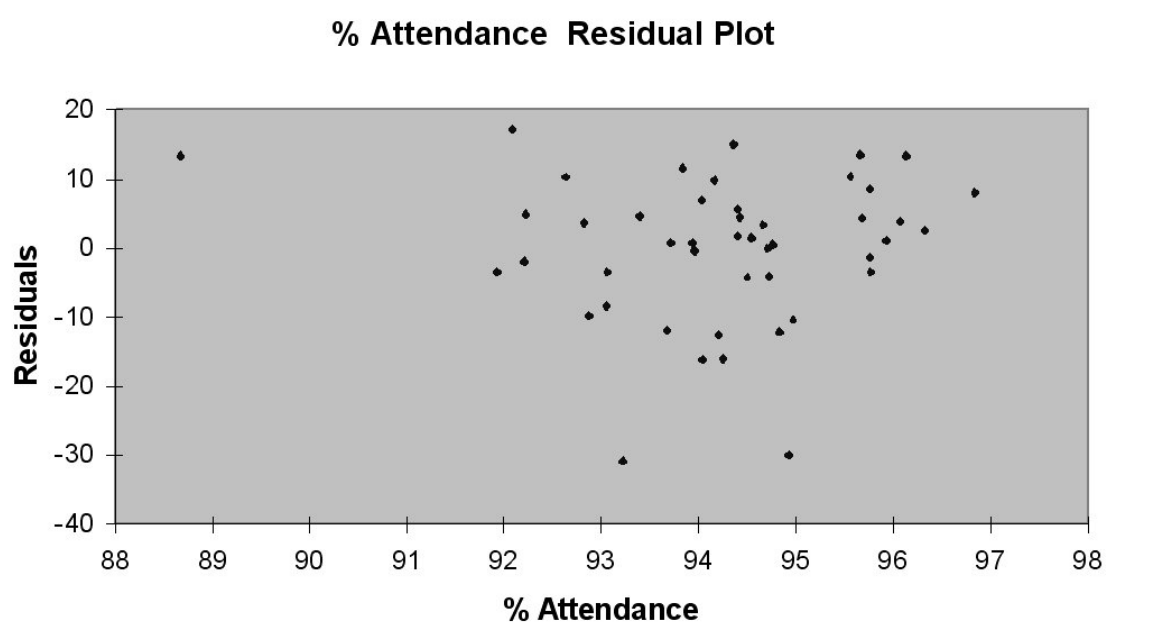



Following is the output of several multiple regression models:

$\text {Model (I) :}$
$\begin{array}{lcrclcr}\hline & \text {Coefficients }& \text {Std Error} & \text {Stat } & \text {p-value} & \text { Lower 95\% }& \text { Upper 95\%} \\\hline \text { Intercept} & -753.4225 & 101.1149 & -7.4511 & 2.88 \mathrm{E}-09 & -957.3401 & -549.5050 \\\% \text {Attend }& 8.5014 & 1.0771 & 7.8929 &6.73 \mathrm{E}-10 & 6.3292 & 10.6735 \\ \text {Salary }& 6.85 \mathrm{E}-07 & 0.0006 & 0.0011 & 0.9991 & -0.0013 & 0.0013 \\ \text {Spending} & 0.0060 & 0.0046 & 1.2879 & 0.2047 & -0.0034 & 0.0153 \\\hline\end{array}$


$\text {Model (II) :}$
$\begin{array}{lcccc}\hline & \text {Coefficients} & \text {Standard Error }& \text { t Stat} & \text { p -value } \\\hline \text {Intercept }& -753.4086 & 99.1451 & -7.5991 & 1.5291 \mathrm{E}-09 \\\% \text {Attendance} & 8.5014 & 1.0645 & 7.9862 & 4.223 \mathrm{E}-10 \\ \text {Spending} & 0.0060 & 0.0034 & 1.7676 & 0.0840 \\\hline\end{array}$


$\text {Model (III) :}$
$\begin{array}{lrrrrl}\hline & \text { d f } & \text { SS } & \text { MS } & \text { F } & \text { Significance F } \\\hline \text { Regression} & 2 & 8162.9429 & 4081.4714 & 39.8708 &1.3201 \mathrm{E}-10 \\ \text { Residual} & 44 & 4504.1635 & 102.3674 & & \\ \text { Total} & 46 & 12667.1064 & & & \\\hline\end{array}$


$\begin{array}{lrcrr}\hline & \text {Coefficients }& \text {Standard Error} & \text { t Stat }& \text {p -value} \\\hline \text {Intercept }& 6672.8367 & 3267.7349 & 2.0420 & 0.0472 \\\% \text { Attendance} & -150.5694 & 69.9519 & -2.1525 & 0.0369 \\\% \text {Attendance Squared}& 0.8532 & 0.3743 & 2.2792 & 0.0276 \\\hline\end{array}$




-Referring to Table 15-8, the "best" model using a 5% level of significance among those chosen by the C_p statistic is

• A) X₁, X₂, X₃.
• B) X₁, X₃.
• C) either of the above
• D) none of the above

---

Definitions:

Underground Prison Economy

A clandestine system of trade and services operated by inmates within a correctional facility.

Illicit Profits

Gains derived unlawfully from criminal activities or unethical business practices.

Prison Officers

Corrections personnel responsible for the supervision, safety, and security of prisoners in a prison, jail, or similar form of detention facility.

Misuse of Authority

The inappropriate or unethical exercise of power by someone in a position of authority.