TABLE 15- 8
the Superintendent of a School District Wanted

question 50

Multiple Choice

TABLE 15- 8
The superintendent of a school district wanted to predict the percentage of students passing a sixth- grade proficiency test. She obtained the data on percentage of students passing the proficiency test (% Passing) , daily average of the percentage of students attending class (% Attendance) , average teacher salary in dollars (Salaries) , and instructional spending per pupil in dollars (Spending) of 47 schools in the state.
Let Y = % Passing as the dependent variable, X₁ = % Attendance, X₂ = Salaries and X₃ = Spending.
The coefficient of multiple determination (R ² _j) of each of the 3 predictors with all the other remaining predictors are,

respectively, 0.0338, 0.4669, and 0.4743.
The output from the best- subset regressions is given below:
Adjusted
$\begin{array}{llcclcc} & & & && \text {Adjusted} \\\text {Model }&\text { Variables} & \mathrm{Cp} & \mathrm{k} &\text {R Square} & \text {R Square} & \text {Std. Error }\\\hline 1 & X1 & 3.05 & 2 & 0.6024 & 0.5936 & 10.5787 \\2 & X1X2 & 3.66 & 3 & 0.6145 & 0.5970 & 10.5350 \\3 & X1X2X3 & 4.00 & 4 & 0.6288 & 0.6029 & 10.4570 \\4 & X1X3 & 2.00 & 3 & 0.6288 & 0.6119 & 10.3375 \\5 & X2 & 67.35 & 2 & 0.0474 & 0.0262 & 16.3755 \\6 & X2X3 & 64.30 & 3 & 0.0910 & 0.0497 & 16.1768 \\7 & X3 & 62.33 & 2 & 0.0907 & 0.0705 & 15.9984 \\\hline\end{array}$

Following is the residual plot for % Attendance: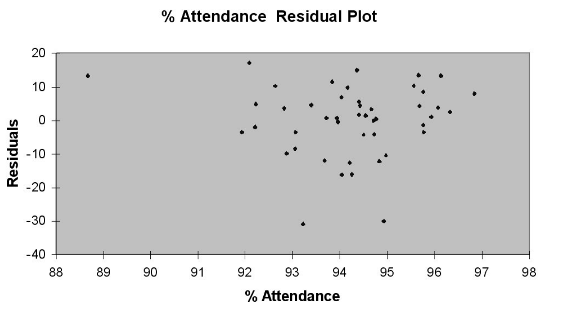



Following is the output of several multiple regression models:

$\text {Model (I) :}$
$\begin{array}{lcrclcr}\hline & \text {Coefficients }& \text {Std Error} & \text {Stat } & \text {p-value} & \text { Lower 95\% }& \text { Upper 95\%} \\\hline \text { Intercept} & -753.4225 & 101.1149 & -7.4511 & 2.88 \mathrm{E}-09 & -957.3401 & -549.5050 \\\% \text {Attend }& 8.5014 & 1.0771 & 7.8929 &6.73 \mathrm{E}-10 & 6.3292 & 10.6735 \\ \text {Salary }& 6.85 \mathrm{E}-07 & 0.0006 & 0.0011 & 0.9991 & -0.0013 & 0.0013 \\ \text {Spending} & 0.0060 & 0.0046 & 1.2879 & 0.2047 & -0.0034 & 0.0153 \\\hline\end{array}$


$\text {Model (II) :}$
$\begin{array}{lcccc}\hline & \text {Coefficients} & \text {Standard Error }& \text { t Stat} & \text { p -value } \\\hline \text {Intercept }& -753.4086 & 99.1451 & -7.5991 & 1.5291 \mathrm{E}-09 \\\% \text {Attendance} & 8.5014 & 1.0645 & 7.9862 & 4.223 \mathrm{E}-10 \\ \text {Spending} & 0.0060 & 0.0034 & 1.7676 & 0.0840 \\\hline\end{array}$


$\text {Model (III) :}$
$\begin{array}{lrrrrl}\hline & \text { d f } & \text { SS } & \text { MS } & \text { F } & \text { Significance F } \\\hline \text { Regression} & 2 & 8162.9429 & 4081.4714 & 39.8708 &1.3201 \mathrm{E}-10 \\ \text { Residual} & 44 & 4504.1635 & 102.3674 & & \\ \text { Total} & 46 & 12667.1064 & & & \\\hline\end{array}$


$\begin{array}{lrcrr}\hline & \text {Coefficients }& \text {Standard Error} & \text { t Stat }& \text {p -value} \\\hline \text {Intercept }& 6672.8367 & 3267.7349 & 2.0420 & 0.0472 \\\% \text { Attendance} & -150.5694 & 69.9519 & -2.1525 & 0.0369 \\\% \text {Attendance Squared}& 0.8532 & 0.3743 & 2.2792 & 0.0276 \\\hline\end{array}$


-Referring to Table 15-8, the "best" model chosen using the adjusted R-square statistic is

• A) X1, X2, X3.
• B) X1, X3.
• C) either of the above
• D) none of the above

---

Definitions:

Subconscious

Part of the mind that is not currently in focal awareness but can influence thoughts and behaviors.

Consciousness Layers

Different levels or aspects of consciousness, ranging from basic awareness to higher states of cognitive functioning.

Freud

Sigmund Freud, an Austrian neurologist and the founder of psychoanalysis, a clinical method for treating psychopathology through dialogue between a patient and a psychoanalyst.

Conscience

An inner feeling or voice viewed as acting as a guide to the rightness or wrongness of one's behavior.