TABLE 15- 8
the Superintendent of a School District Wanted

question 32

Multiple Choice

TABLE 15- 8
The superintendent of a school district wanted to predict the percentage of students passing a sixth- grade proficiency test. She obtained the data on percentage of students passing the proficiency test (% Passing) , daily average of the percentage of students attending class (% Attendance) , average teacher salary in dollars (Salaries) , and instructional spending per pupil in dollars (Spending) of 47 schools in the state.
Let Y = % Passing as the dependent variable, X₁ = % Attendance, X₂ = Salaries and X₃ = Spending.
The coefficient of multiple determination (R ² _j) of each of the 3 predictors with all the other remaining predictors are,

respectively, 0.0338, 0.4669, and 0.4743.
The output from the best- subset regressions is given below:

$\begin{array}{llcclcc} & & & && \text {Adjusted} \\\text {Model }&\text { Variables} & \mathrm{Cp} & \mathrm{k} &\text {R Square} & \text {R Square} & \text {Std. Error }\\\hline 1 & X1 & 3.05 & 2 & 0.6024 & 0.5936 & 10.5787 \\2 & X1X2 & 3.66 & 3 & 0.6145 & 0.5970 & 10.5350 \\3 & X1X2X3 & 4.00 & 4 & 0.6288 & 0.6029 & 10.4570 \\4 & X1X3 & 2.00 & 3 & 0.6288 & 0.6119 & 10.3375 \\5 & X2 & 67.35 & 2 & 0.0474 & 0.0262 & 16.3755 \\6 & X2X3 & 64.30 & 3 & 0.0910 & 0.0497 & 16.1768 \\7 & X3 & 62.33 & 2 & 0.0907 & 0.0705 & 15.9984 \\\hline\end{array}$

Following is the residual plot for % Attendance: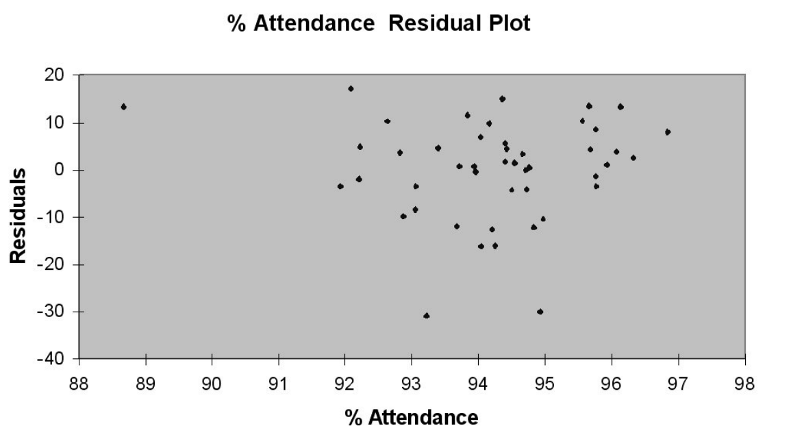



Following is the output of several multiple regression models:

$\text {Model (I) :}$
$\begin{array}{lcrclcr}\hline & \text {Coefficients }& \text {Std Error} & \text {Stat } & \text {p-value} & \text { Lower 95\% }& \text { Upper 95\%} \\\hline \text { Intercept} & -753.4225 & 101.1149 & -7.4511 & 2.88 \mathrm{E}-09 & -957.3401 & -549.5050 \\\% \text {Attend }& 8.5014 & 1.0771 & 7.8929 &6.73 \mathrm{E}-10 & 6.3292 & 10.6735 \\ \text {Salary }& 6.85 \mathrm{E}-07 & 0.0006 & 0.0011 & 0.9991 & -0.0013 & 0.0013 \\ \text {Spending} & 0.0060 & 0.0046 & 1.2879 & 0.2047 & -0.0034 & 0.0153 \\\hline\end{array}$


$\text {Model (II) :}$
$\begin{array}{lcccc}\hline & \text {Coefficients} & \text {Standard Error }& \text { t Stat} & \text { p -value } \\\hline \text {Intercept }& -753.4086 & 99.1451 & -7.5991 & 1.5291 \mathrm{E}-09 \\\% \text {Attendance} & 8.5014 & 1.0645 & 7.9862 & 4.223 \mathrm{E}-10 \\ \text {Spending} & 0.0060 & 0.0034 & 1.7676 & 0.0840 \\\hline\end{array}$


$\text {Model (III) :}$
$\begin{array}{lrrrrl}\hline & \text { d f } & \text { SS } & \text { MS } & \text { F } & \text { Significance F } \\\hline \text { Regression} & 2 & 8162.9429 & 4081.4714 & 39.8708 &1.3201 \mathrm{E}-10 \\ \text { Residual} & 44 & 4504.1635 & 102.3674 & & \\ \text { Total} & 46 & 12667.1064 & & & \\\hline\end{array}$


$\begin{array}{lrcrr}\hline & \text {Coefficients }& \text {Standard Error} & \text { t Stat }& \text {p -value} \\\hline \text {Intercept }& 6672.8367 & 3267.7349 & 2.0420 & 0.0472 \\\% \text { Attendance} & -150.5694 & 69.9519 & -2.1525 & 0.0369 \\\% \text {Attendance Squared}& 0.8532 & 0.3743 & 2.2792 & 0.0276 \\\hline\end{array}$




-Referring to Table 15-8, which of the following models should be taken into consideration using the Mallows' Cp statistic?

• A) X₁, X₂, X₃
• B) X₁, X₃
• C) both of the above
• D) none of the above

---

Definitions:

Rape Trauma Syndrome

A form of post-traumatic stress disorder specifically associated with the traumatic experience of rape, characterized by acute phases and long-term reorganization of lifestyle.

Depression

A mental health disorder characterized by persistently depressed mood or loss of interest in activities, causing significant impairment in daily life.

Rage

An intense, uncontrolled anger that often manifests in aggressive or violent behavior.

Continuing Anxiety

Persistent feelings of worry, nervousness, or unease about something with an uncertain outcome.