TABLE 15-9
Many factors determine the attendance at Major League Baseball games. These factors can include when the game is played, the weather, the opponent, whether or not the team is having a good season, and whether or not a marketing promotion is held. Data from 80 games of the Kansas City Royals for the following variables are collected.
ATTENDANCE = Paid attendance for the game
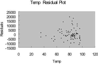
TEMP = High temperature for the day
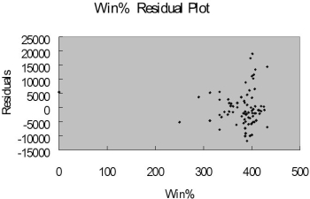
WIN% = Team's winning percentage at the time of the game
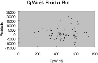
OPWIN% = Opponent team's winning percentage at the time of the game WEEKEND - 1 if game played on Friday, Saturday or Sunday; 0 otherwise
PROMOTION - 1 = if a promotion was held; 0 = if no promotion was held
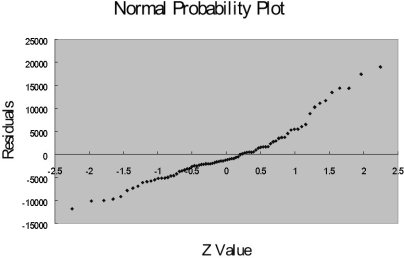
The regression results using attendance as the dependent variable and the remaining five variables as the independent variables are presented below.
The coefficient of multiple determination ( R 2 j) of each of the 5 predictors with all the other remaining predictors are, respectively, 0.2675, 0.3101, 0.1038, 0.7325, and 0.7308.
-Referring to Table 15-9, which of the following assumptions is most likely violated based on the residual plot for WIN%?
Definitions:
Specific Customers
This refers to identified individual or business customers with unique needs or characteristics that a company targets or serves.
Direct Write-off Method
An accounting method where uncollectible debts are written off as an expense only when they are confirmed to be uncollectible.
Materiality Constraint
An accounting principle that allows for ignoring minor discrepancies that would not affect the decision-making process of users of financial statements.
Uncollectible Account Receivable
An accounting term for receivables from sales that are considered not collectible, resulting in a bad debt expense.
Q2: Referring to Table 18-8, based on the
Q3: Referring to Table 14-15, the fitted model
Q26: Collinearity is present if the dependent variable
Q72: Referring to Table 15-9, what is the
Q75: Referring to Table 16-15, what is the
Q95: Referring to Table 14-11, which of the
Q103: Which of the following statements about moving
Q159: Referring to Table 13-12, the value of
Q183: Referring to Table 14-17, what is the
Q236: Referring to Table 14-9, if variables that