TABLE 15-9
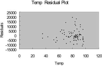
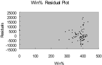
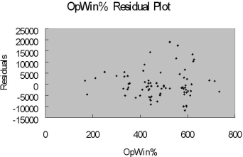
Many factors determine the attendance at Major League Baseball games. These factors can include when the game is played, the weather, the opponent, whether or not the team is having a good season, and whether or not a marketing promotion is held. Data from 80 games of the Kansas City Royals for the following variables are collected.
ATTENDANCE = Paid attendance for the game
TEMP = High temperature for the day
WIN% = Team's winning percentage at the time of the game
OPWIN% = Opponent team's winning percentage at the time of the game WEEKEND - 1 if game played on Friday, Saturday or Sunday; 0 otherwise PROMOTION - 1 = if a promotion was held; 0 = if no promotion was held
The regression results using attendance as the dependent variable and the remaining five variables as the independent variables are presented below.
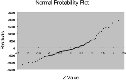
The coefficient of multiple determination ( R 2 j) of each of the 5 predictors with all the other remaining predictors are, respectively, 0.2675, 0.3101, 0.1038, 0.7325, and 0.7308.
-Referring to Table 15-9, what is the correct interpretation for the estimated coefficient for PROMOTION?
Definitions:
Western Front
The main theatre of war during World War I, stretching from the North Sea to the Swiss border, where most of the fighting between Germany and the Allies occurred.
Yalta Conference
A 1945 meeting between Churchill, Roosevelt, and Stalin to discuss the post-World War II reorganization of Europe and the establishment of the United Nations.
Great Britain
An island in the North Atlantic Ocean off the northwest coast of continental Europe, comprising the countries of England, Scotland, and Wales.
United States
A federal republic in North America comprising 50 states and a federal district, known for its democratic governance and diverse population.
Q9: If the correlation coefficient (r) = 1.00,
Q43: Referring to Table 14-1, if an employee
Q61: A professor of economics at a small
Q62: Referring to Table 14-3, to test whether
Q111: Referring to Table 17-1, if the probability
Q115: Blossom's Flowers purchases roses for sale for
Q127: Referring to Table 17-5, what is the
Q137: Referring to Table 13-5, the prediction for
Q154: Referring to Table 16-7, the number of
Q158: Referring to Table 16-15, what is the