TABLE 15-9
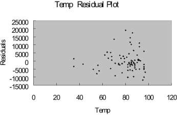
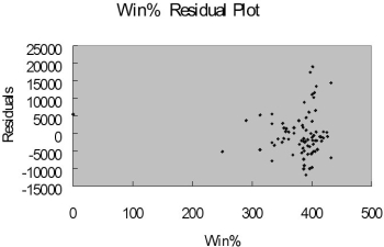
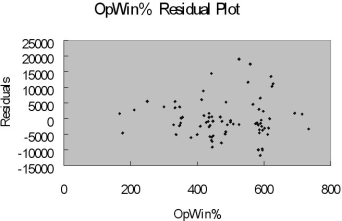
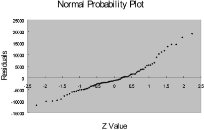
Many factors determine the attendance at Major League Baseball games. These factors can include when the game is played, the weather, the opponent, whether or not the team is having a good season, and whether or not a marketing promotion is held. Data from 80 games of the Kansas City Royals for the following variables are collected.
ATTENDANCE = Paid attendance for the game
TEMP = High temperature for the day
WIN% = Team's winning percentage at the time of the game
OPWIN% = Opponent team's winning percentage at the time of the game WEEKEND - 1 if game played on Friday, Saturday or Sunday; 0 otherwise PROMOTION - 1 = if a promotion was held; 0 = if no promotion was held
The regression results using attendance as the dependent variable and the remaining five variables as the independent variables are presented below.
The coefficient of multiple determination ( R 2 j ) of each of the 5 predictors with all the other remaining predictors are,
respectively, 0.2675, 0.3101, 0.1038, 0.7325, and 0.7308.
-Referring to Table 15-9,_______ of the variation in ATTENDANCE can be explained by the five independent variables.
Definitions:
Future Value
The value of an asset or cash at a specific future date, based on its expected growth over time.
Compounded Monthly
Interest calculation method where the accrued interest is added to the principal sum each month, leading to interest on interest.
Interest Charge
A fee charged by a lender to a borrower for the use of borrowed money, often expressed as an annual percentage of the principal.
Inherited Money
Wealth or assets received from someone after their death.
Q11: Referring to Table 18-5, a p control
Q12: Referring to Table 16-12, using the second-order
Q13: Referring to Table 16-14, what are the
Q21: Referring to Table 15-9, there is reason
Q61: Referring to Table 16-5, in testing the
Q69: Referring to Table 14-10, the estimated average
Q75: Referring to Table 18-1, what is the
Q79: Given a data set with 15 yearly
Q107: Referring to Table 14-11, there is not
Q172: Referring to Table 14-15, the fitted model