SCENARIO 17-2 One of the most common questions of prospective house buyers pertains to the cost of heating in dollars (Y) . To provide its customers with information on that matter, a large real estate firm used the following 4 variables to predict heating costs: the daily minimum outside temperature in degrees of Fahrenheit (X1) , the amount of insulation in inches (X2) , the number of windows in the house (X3) , and the age of the furnace in years (X4) . Given below are the EXCEL outputs of two regression models.
Model 1
Regression Statistics R Square Adjusted R Square Observations 0.80800.756820 ANOVA
Regression Residual Total df41519 SS 169503.424140262.3259209765.75MS42375.862684.155F15.7874 Significance F0.0000
Intereept X1 (Temperature) X2 (Insulation) X3 (Windows) X4 (Furnace Age) Coefficients 421.4277−4.5098−14.90290.21516.3780 Standard Error 77.86140.81295.05084.86754.1026 t Stat 5.4125−5.5476−2.95050.04421.5546 P-value 0.00000.00000.00990.96530.1408 Lower 90.0% 284.9327−5.9349−23.7573−8.3181−0.8140 Upper 90.0% 557.9227−3.0847−6.04858.748413.5702
Model 2
Regression Statistics R Square Adjusted R Square Observations 0.77680.750620
ANOVA
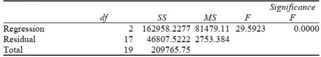
Intercept X1 (Temperature) X2 (Insulation) Coefficients 489.3227−5.1103−14.7195 Standard Error 43.98260.69514.8864t Stat 11.1253−7.3515−3.0123 P-value 0.00000.00000.0078 Lower 95% 396.5273−6.5769−25.0290 Upper 95% 582.1180−3.6437−4.4099
-Referring to Scenario 17-2, what can we say about Model 1?
Antihistamine
A type of medication that counteracts the effects of histamine, improving allergy symptoms.
Inflammation
A biological response to harmful stimuli such as pathogens, damaged cells, or irritants, characterized by redness, swelling, heat, pain, and often loss of function.
Immunoglobulin
Proteins in the blood plasma produced by B cells that act as antibodies to help fight infections.