SCENARIO 17-10 Given Below Are Results from the Regression Analysis $1 =$

question 278

True/False

SCENARIO 17-10 Given below are results from the regression analysis where the dependent variable is the number of weeks a worker is unemployed due to a layoff (Unemploy) and the independent variables are the age of the worker (Age), the number of years of education received (Edu), the number of years at the previous job (Job Yr), a dummy variable for marital status (Married: $1 =$ married, $0 =$ otherwise), a dummy variable for head of household (Head: $1 =$ yes, $0 =$ no) and a dummy variable for management position (Manager: $1 =$ yes, $0 =$ no). We shall call this Model 1. The coefficient of partial determination ( $R _ { \mathrm { y } } ^ { 2 }$ (All raiables excopt $j$ ) ) of each of the 6 predictors are, respectively, $0.2807$ , $0.0386,0.0317,0.0141,0.0958$ , and $0.1201$ .

$\begin{array}{lr}\hline{\text { Regression Statistics }} \\\hline \text { Multiple R } & 0.7035 \\\text { R Square } & 0.4949 \\\text { Adjusted R } & 0.4030 \\\text { Square } & \\\text { Standard } & 18.4861 \\\text { Error } & \\\text { Observations } & 40 \\\hline\end{array}$
$\text { ANOVA }$



$$\begin{array}{l}\begin{array} { l r r r r r r } \hline & \text { Coefficients } & \text { Standard Error } & { t \text { Stat } } & \text { P-value } & \text { Lower 95\% } & \text { Upper 95\% } \\\hline \text { Intercept } & 32.6595 & 23.18302 & 1.4088 & 0.1683 & - 14.5067 & 79.8257 \\\text { Age } & 1.2915 & 0.3599 & 3.5883 & 0.0011 & 0.5592 & 2.0238 \\\text { Edu } & - 1.3537 & 1.1766 & - 1.1504 & 0.2582 & - 3.7476 & 1.0402 \\\text { Job Yr } & 0.6171 & 0.5940 & 1.0389 & 0.3064 & - 0.5914 & 1.8257 \\\text { Married } & - 5.2189 & 7.6068 & - 0.6861 & 0.4974 & - 20.6950 & 10.2571 \\\text { Head } & - 14.2978 & 7.6479 & - 1.8695 & 0.0704 & - 29.8575 & 1.2618 \\\text { Manager } & - 24.8203 & 11.6932 & - 2.1226 & 0.0414 & - 48.6102 & - 1.0303 \\\hline\end{array}\end{array}$$
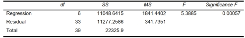
-Referring to Scenario 17-10 Model 1, the null hypothesis should be rejected at a
10% level of significance when testing whether being married or not makes a difference in the
mean number of weeks a worker is unemployed due to a layoff while holding constant the effect
of all the other independent variables.

---

Definitions:

Positive Profits

Earnings that exceed the costs and expenses incurred to generate those earnings.

Price Elastic

Refers to the sensitivity of the quantity demanded of a good to a change in its price; high elasticity indicates that demand varies significantly with price.

Brand X Burger

A fictional or hypothetical brand used to discuss marketing, product differentiation, or consumer preference scenarios.

Demand For Food

Demand For Food describes the quantity of food products that consumers are willing and able to purchase at various price levels, usually influenced by factors like income, taste, and price.