SCENARIO 17-10 Given Below Are Results from the Regression Analysis $1 =$

question 295

True/False

SCENARIO 17-10 Given below are results from the regression analysis where the dependent variable is the number of weeks a worker is unemployed due to a layoff (Unemploy) and the independent variables are the age of the worker (Age), the number of years of education received (Edu), the number of years at the previous job (Job Yr), a dummy variable for marital status (Married: $1 =$ married, $0 =$ otherwise), a dummy variable for head of household (Head: $1 =$ yes, $0 =$ no) and a dummy variable for management position (Manager: $1 =$ yes, $0 =$ no). We shall call this Model 1. The coefficient of partial determination ( $R _ { \mathrm { y } } ^ { 2 }$ (All raiables excopt $j$ ) ) of each of the 6 predictors are, respectively, $0.2807$ , $0.0386,0.0317,0.0141,0.0958$ , and $0.1201$ .

$\begin{array}{lr}\hline{\text { Regression Statistics }} \\\hline \text { Multiple R } & 0.7035 \\\text { R Square } & 0.4949 \\\text { Adjusted R } & 0.4030 \\\text { Square } & \\\text { Standard } & 18.4861 \\\text { Error } & \\\text { Observations } & 40 \\\hline\end{array}$
$\text { ANOVA }$



$$\begin{array}{l}\begin{array} { l r r r r r r } \hline & \text { Coefficients } & \text { Standard Error } & { t \text { Stat } } & \text { P-value } & \text { Lower 95\% } & \text { Upper 95\% } \\\hline \text { Intercept } & 32.6595 & 23.18302 & 1.4088 & 0.1683 & - 14.5067 & 79.8257 \\\text { Age } & 1.2915 & 0.3599 & 3.5883 & 0.0011 & 0.5592 & 2.0238 \\\text { Edu } & - 1.3537 & 1.1766 & - 1.1504 & 0.2582 & - 3.7476 & 1.0402 \\\text { Job Yr } & 0.6171 & 0.5940 & 1.0389 & 0.3064 & - 0.5914 & 1.8257 \\\text { Married } & - 5.2189 & 7.6068 & - 0.6861 & 0.4974 & - 20.6950 & 10.2571 \\\text { Head } & - 14.2978 & 7.6479 & - 1.8695 & 0.0704 & - 29.8575 & 1.2618 \\\text { Manager } & - 24.8203 & 11.6932 & - 2.1226 & 0.0414 & - 48.6102 & - 1.0303 \\\hline\end{array}\end{array}$$
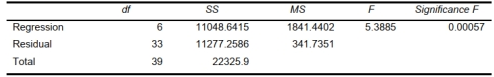
-Referring to Scenario 17-10 Model 1, there is sufficient evidence that being
married or not makes a difference in the mean number of weeks a worker is unemployed due to a
layoff while holding constant the effect of all the other independent variables at a 10% level of
significance.

---

Definitions:

Variable Resources

Inputs used in production that can be adjusted in the short term to meet changes in output levels, such as labor and raw materials.

AVC Curve

Represents the average variable cost of production plotted against the quantity of output, showing how variable costs per unit change with changes in output.

MC Curve

Short for Marginal Cost Curve, it represents the change in total cost that arises when the quantity produced is incremented by one unit.

Marginal Cost

The increase in cost that arises from producing one additional unit of a good or service.