SCENARIO 17-10 Given Below Are Results from the Regression Analysis $1 =$

question 21

True/False

SCENARIO 17-10 Given below are results from the regression analysis where the dependent variable is the number of weeks a worker is unemployed due to a layoff (Unemploy) and the independent variables are the age of the worker (Age), the number of years of education received (Edu), the number of years at the previous job (Job Yr), a dummy variable for marital status (Married: $1 =$ married, $0 =$ otherwise), a dummy variable for head of household (Head: $1 =$ yes, $0 =$ no) and a dummy variable for management position (Manager: $1 =$ yes, $0 =$ no). We shall call this Model 1. The coefficient of partial determination ( $R _ { \mathrm { y } } ^ { 2 }$ (All raiables excopt $j$ ) ) of each of the 6 predictors are, respectively, $0.2807$ , $0.0386,0.0317,0.0141,0.0958$ , and $0.1201$ .

$\begin{array}{lr}\hline{\text { Regression Statistics }} \\\hline \text { Multiple R } & 0.7035 \\\text { R Square } & 0.4949 \\\text { Adjusted R } & 0.4030 \\\text { Square } & \\\text { Standard } & 18.4861 \\\text { Error } & \\\text { Observations } & 40 \\\hline\end{array}$
$\text { ANOVA }$



$$\begin{array}{l}\begin{array} { l r r r r r r } \hline & \text { Coefficients } & \text { Standard Error } & { t \text { Stat } } & \text { P-value } & \text { Lower 95\% } & \text { Upper 95\% } \\\hline \text { Intercept } & 32.6595 & 23.18302 & 1.4088 & 0.1683 & - 14.5067 & 79.8257 \\\text { Age } & 1.2915 & 0.3599 & 3.5883 & 0.0011 & 0.5592 & 2.0238 \\\text { Edu } & - 1.3537 & 1.1766 & - 1.1504 & 0.2582 & - 3.7476 & 1.0402 \\\text { Job Yr } & 0.6171 & 0.5940 & 1.0389 & 0.3064 & - 0.5914 & 1.8257 \\\text { Married } & - 5.2189 & 7.6068 & - 0.6861 & 0.4974 & - 20.6950 & 10.2571 \\\text { Head } & - 14.2978 & 7.6479 & - 1.8695 & 0.0704 & - 29.8575 & 1.2618 \\\text { Manager } & - 24.8203 & 11.6932 & - 2.1226 & 0.0414 & - 48.6102 & - 1.0303 \\\hline\end{array}\end{array}$$
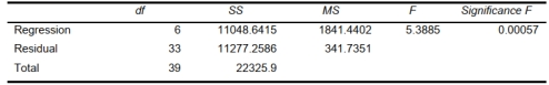
-Referring to Scenario 17-10 Model 1, we can conclude that, holding constant the
effect of the other independent variables, the number of years of education received has no impact
on the mean number of weeks a worker is unemployed due to a layoff at a 1% level of
significance if all we have is the information of the 95% confidence interval estimate for?2 .

---

Definitions:

Resource Prices

Refers to the costs associated with inputs used in the production of goods or services, such as raw materials, labor, and capital.

Market Demand

The total quantity of a product or service that all consumers in a market are willing and able to purchase at various prices.

Increases

This term refers to a situation where a quantity or quality of something goes up or becomes more.

Constant-Cost Industry

An industry where the costs of production do not change as the overall level of production increases or decreases.