Here are data about the average January low temperature in cities in the United States, and factors that might allow us to
predict temperature. The data, available for 55 cities, include: 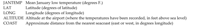 We will attempt to make a regression model to help account for mean January temperature and to understand the effects of
the various predictors.
At each step of the analysis you may assume that things learned earlier in the process are known.
Units Note: The "degrees" of temperature, given here on the Fahrenheit scale, have only coincidental language relationship to
the "degrees" of longitude and latitude. The geographic "degrees" are based on modeling the Earth as a sphere and dividing it
up into 360 degrees for a full circle. Thus 180 degrees of longitude is halfway around the world from Greenwich, England
(0°) and Latitude increases from 0 degrees at the Equator to 90 degrees of (North) latitude at the North Pole. 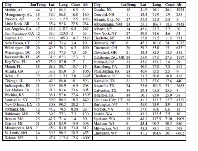
-It is possible that the distance that a city is from the ocean could affect its average January
low temperature. Coast gives an approximate distance of each city from the East Coast or
West Coast (whichever is nearer). Including it in the regression yields the following
regression table: Dependent variable is:JanTemp
R squared squared (adjusted) with degrees of freedom
And here is a scatterplot of the residuals: 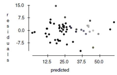
Definitions:
Satisfying Content
Content that fulfills or exceeds the expectations and needs of the intended audience, often used in the context of media and digital marketing.
Wage Discrimination
The practice of paying employees differently for the same work based on gender, race, age, or other non-performance-related factors.
Seniority System
A system in a workplace where employee benefits such as promotions and layoffs are determined based on the length of service.
Strategic Objectives
High-level goals aligned with an organization's mission and vision, focused on achieving long-term success.
Q4: When a sum of squares is divided
Q5: Nationalities of survey respondents.<br>A) Nominal<br>B) Ratio<br>C) Ordinal<br>D)
Q5: Trainers need to estimate the level of
Q22: A T.V. show's executives raised the fee
Q28: What alpha level did the group use?
Q44: A consultant talked the group into gathering
Q45: A college student wants to purchase one
Q105: The principal of a small elementary school
Q110: Suppose that our fearless fisherman goes out
Q127: The normal monthly precipitation (in inches)