A college admissions counselor was interested in finding out how well high school grade point averages (HS GPA) predict first-year college GPAs (FY GPA). A random sample of data from first-year students was reviewed to obtain high school and first-year college GPAs. The data are shown below:
Dependent variable is: FY GPA
No Selector
squared squared (adjusted)
with degrees of freedom
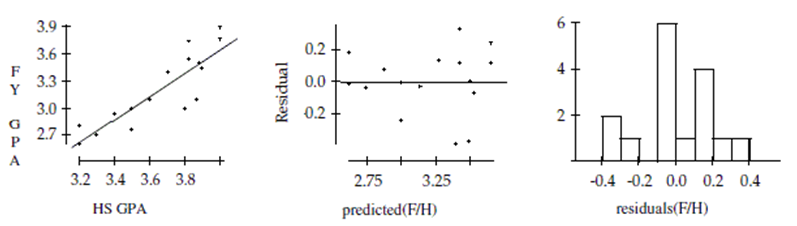
-Create and interpret a 95% confidence interval for the slope of the regression line.
Definitions:
Manufacturing Cost Variance
The difference between the actual costs of production and the standard or expected costs, indicating efficiency or inefficiency in the manufacturing process.
Direct Materials Cost Variance
The difference between the actual cost of direct materials used in production and the standard cost expected to be used.
Direct Labor Cost Variance
The difference between the budgeted cost of direct labor and the actual cost incurred.
Cost Variance
The difference between the expected (budgeted) cost and the actual cost incurred.
Q8: Which is true of the data shown
Q67: In a local school, vending machines
Q80: Which of the following are NOT characteristics
Q114: Do you think a linear model is
Q145: A professor was curious about her
Q199: If we wish to compare the average
Q322: Describe an advantage of the placebo.
Q487: All but one of these statements contain
Q553: All but one of the statements
Q751: Explain what 90% confidence means in this