SCENARIO 15-4 the Superintendent of a School District Wanted to Predict

question 36

Multiple Choice

SCENARIO 15-4 The superintendent of a school district wanted to predict the percentage of students passing a sixth-grade proficiency test.She obtained the data on percentage of students passing the proficiency test (% Passing) , daily mean of the percentage of students attending class (% Attendance) , mean teacher salary in dollars (Salaries) , and instructional spending per pupil in dollars (Spending) of 47 schools in the state. Let Y = % Passing as the dependent variable, Attendance, Salaries and Spending. The coefficient of multiple determination ( ) of each of the 3 predictors with all the other remaining predictors are, respectively, 0.0338, 0.4669, and 0.4743. The output from the best-subset regressions is given below: 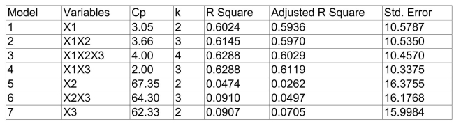Following is the residual plot for % Attendance: 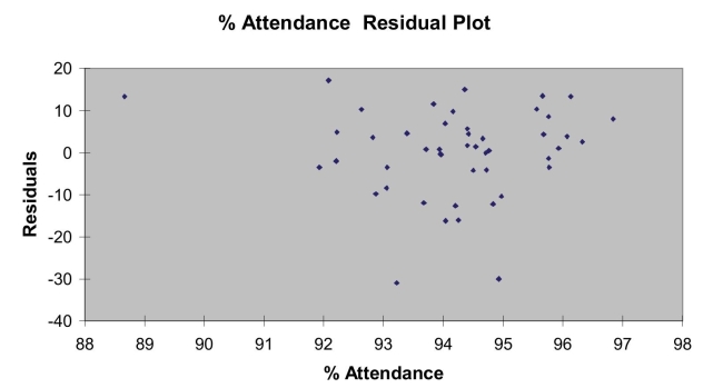Following is the output of several multiple regression models:
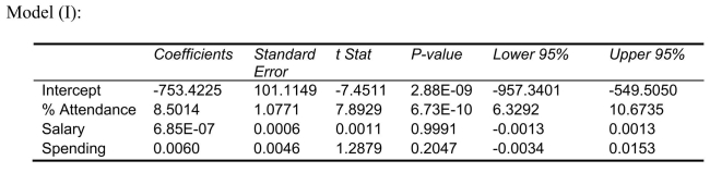
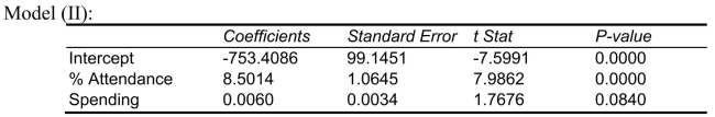
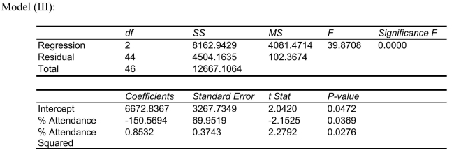
-Referring to Scenario 15-4, the better model using a 5% level of significance derived from the "best" model above is

---

Definitions:

Consumer Surplus

The benefit obtained by consumers because they are able to purchase a product for a price that is less than the highest price that they would be willing to pay.

Optimal Consumption

refers to the situation in which a consumer allocates their income in a way that maximizes their overall satisfaction or utility, given their preferences and the prices of goods and services.

Demand Schedule

A demand schedule is a table that shows the quantity of a good or service that consumers are willing and able to purchase at various prices.

Price Elasticity

A measure of how much the quantity demanded of a good responds to a change in the price of that good.