Quarterly sales of a department store for the last seven years are given in the following table. 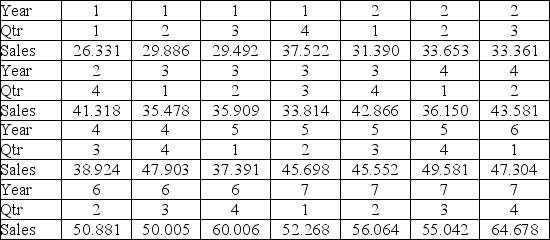
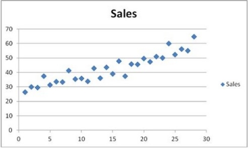 The scatterplot shows that the quarterly sales have an increasing trend and seasonality. A linear regression model given by Sales = β0 + β1Qtr1 + β2Qtr2 + β3Qtr3 + β4t + ε, where t is the time period (t = 1, ..., 28) and Qtr1, Qtr2, and Qtr3 are quarter dummies, is estimated and then used to make forecasts. For the regression model, the following partial output is available.
  Using MSE and MAD, compare the linear trend equation with seasonal dummy variables,
  t = 31,9261 - 7.855Qtr1 - 4.7362Qtr2 - 7.1656Qtr3 + 1.0749t, and the decomposition method equation
  t =
t =  t ×
t ×  t with
  t = 26.8819 + 1.0780t and the quarterly seasonal indices: 0.9322, 1.0066, 0.9441, and 1.1171. Which of the two corresponding forecasting models is recommended?
Definitions:
Q28: A realtor wants to predict and compare
Q31: Which of the following equations is a
Q52: Typically, the sales volume declines with an
Q75: The only possible income from an investment
Q78: For the Kruskal-Wallis test with n<sub>i</sub> ≥
Q82: For the Spearman rank correlation test we
Q89: The seller of a put option:<br>A)has the
Q93: Refer to below regression results. <img src="https://d2lvgg3v3hfg70.cloudfront.net/TB6618/.jpg"
Q99: A long straddle is a strategy that
Q109: Investment institutions usually have funds with different