Quarterly sales of a department store for the last seven years are given in the following table. 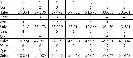
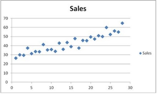 The scatterplot shows that the quarterly sales have an increasing trend and seasonality. A linear regression model given by Sales = β0 + β1Qtr1 + β2Qtr2 + β3Qtr3 + β4t + ε, where t is the time period (t = 1, ..., 28) and Qtr1, Qtr2, and Qtr3 are quarter dummies, is estimated and then used to make forecasts. For the regression model, the following partial output is available.
  Using MSE and MAD, compare the linear trend equation with seasonal dummy variables,
  t = 31,9261 - 7.855Qtr1 - 4.7362Qtr2 - 7.1656Qtr3 + 1.0749t, and the decomposition method equation
  t =
t =  t ×
t ×  t with
  t = 26.8819 + 1.0780t and the quarterly seasonal indices: 0.9322, 1.0066, 0.9441, and 1.1171. Which of the two corresponding forecasting models is recommended?
Definitions:
Occult Blood
Hidden blood in stool or other bodily substances, not visible to the eye but detectable through specific medical tests.
Malabsorption
A disorder where the intestines fail to efficiently absorb nutrients from food, leading to deficiencies and other health issues.
Iron Supplements
Products taken to increase iron levels in the body, often used to treat or prevent iron-deficiency anemia.
Ostomy
A surgical procedure creating an opening in the body for the discharge of body wastes.
Q12: When a time series is analyzed by
Q17: In the quadratic trend model, y<sub>t</sub> =
Q21: If the price index for a particular
Q22: When the decomposition model, y<sub>t</sub> = T<sub>t</sub>
Q64: For the exponential model ln(y) = β<sub>0</sub>
Q83: For the log-log model ln(y) = β<sub>0</sub>
Q95: A researcher has developed the following regression
Q101: A marketing firm needs to replace its
Q109: Which of the following is true of
Q110: Suppose you are long the $32 Aug.NAB