Instruction 12-12
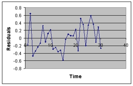
The manager of the purchasing department of a large savings and loan organization would like to develop a model to predict the amount of time (measured in hours) it takes to record a loan application.Data are collected from a sample of 30 days,and the number of applications recorded and completion time in hours is recorded.Below is the regression output:
Note: 4.3946E-15 is 4.3946 x 10⁻¹⁵.
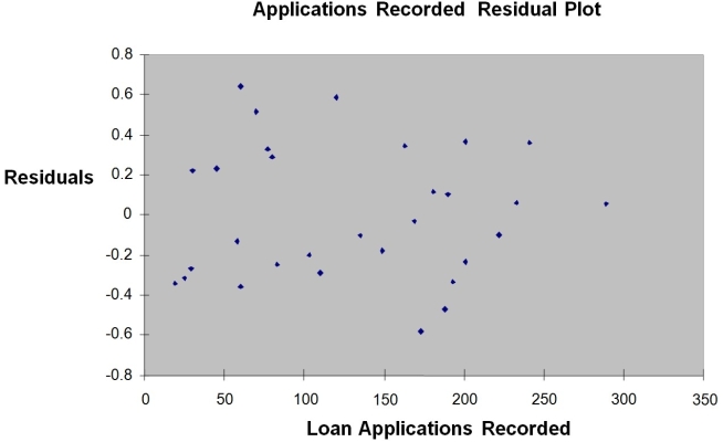
-Referring to Instruction 12-12,the error sum of squares (SSE) of the above regression is
Definitions:
Managed Float
A currency exchange rate policy where a currency's value is allowed to fluctuate in response to foreign exchange market mechanisms, but the central bank may intervene to stabilize the currency if necessary.
Managed Floating
An exchange rate system where a country's currency value is allowed to fluctuate in response to foreign-exchange market mechanisms, but the central bank can intervene to prevent extreme fluctuations.
Bretton Woods System
A monetary management system established post-World War II, which set up rules for commercial and financial relations among major industrial states.
Q1: Referring to Instruction 11-3,the value of the
Q2: Referring to Instruction 13-16 Model 1,you can
Q27: If the correlation coefficient (r)= 1.00,then<br>A)all the
Q43: Referring to Instruction 14-9,the Holt-Winters method for
Q44: Referring to Instruction 12-10,what are the degrees
Q78: Referring to Instruction 12-12,the p-value of the
Q81: Referring to Instruction 10-4,what is(are)the critical value(s)of
Q83: Referring to Instruction 14-11,the estimate of the
Q100: Referring to Instruction 10-2,what is the 95%
Q164: Referring to Instruction 13-6,the estimated value of