The following table shows the annual revenues (in millions of dollars)of a pharmaceutical company over the period 1990-2011. 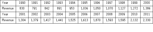 The autoregressive models of order 1 and 2,yt = β0 + β1yt - 1 + εt,and yt = β0 + β1yt - 1 + β2yt - 2 + εt,were applied on the time series to make revenue forecasts.The relevant parts of Excel regression outputs are given below.
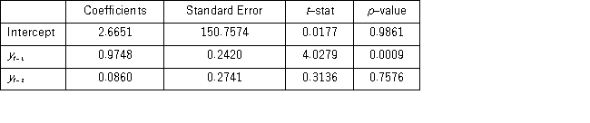
Model AR(1): 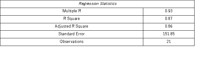
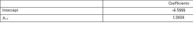 Model AR(2):
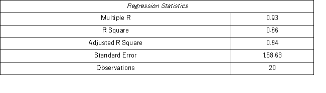
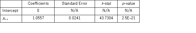
 When for AR(1),H0: β0 = 0 is tested against HA: β0 ≠ 0,the p-value of this t test shown by Excel output is 0.9590.This could suggest that the model yt = β1yt-1 + εt might be an alternative to the AR(1)model yt = β0 + β1yt-1 + εt.Excel partial output for this simplified model is as follows:
 (Use Regression in Data Analysis of Excel. )
Compare the autoregressive models yt = β0 + β1yt-1 + εt;yt = β0 + β1yt-1 + β2yt-2 + εt,andyt = β1yt-1 + εt,through the use of MSE and MAD.
Definitions:
Primary Socialization
Is the process of acquiring the basic skills needed to function in society during childhood. Primary socialization usually takes place in a family.
School
An educational institution where children and young people receive formal education through a structured curriculum.
Resocialization
The process by which one's sense of social values, beliefs, and norms are re-engineered, often in a new social environment.
Hidden Curriculum
The unintended lessons, values, and perspectives that students learn in school, which are not part of the formal curriculum.
Q23: Consider the following regression results based on
Q46: A sociologist wishes to study the relationship
Q70: A bank manager is interested in assigning
Q72: The following table shows the value of
Q86: The following Excel scatterplot with the fitted
Q94: A dummy variable is also referred to
Q113: The major shortcoming of the general linear
Q115: The linear trend, <img src="https://d2lvgg3v3hfg70.cloudfront.net/TB4266/.jpg" alt="The linear
Q119: A real estate analyst believes that the
Q127: An real estate analyst believes that the