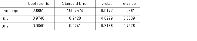
The following table shows the annual revenues (in millions of dollars)of a pharmaceutical company over the period 1990-2011. 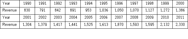 The autoregressive models of order 1 and 2,yt = β0 + β1yt - 1 + εt,and yt = β0 + β1yt - 1 + β2yt - 2 + εt,were applied on the time series to make revenue forecasts.The relevant parts of Excel regression outputs are given below.
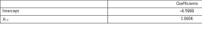
Model AR(1): 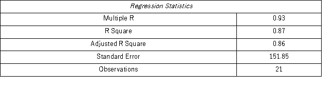
 Model AR(2):
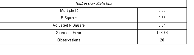
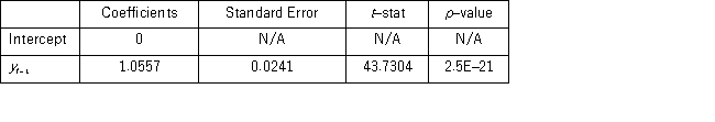
 When for AR(1),H0: β0 = 0 is tested against HA: β0 ≠ 0,the p-value of this t test shown by Excel output is 0.9590.This could suggest that the model yt = β1yt-1 + εt might be an alternative to the AR(1)model yt = β0 + β1yt-1 + εt.Excel partial output for this simplified model is as follows:
 (Use Regression in Data Analysis of Excel. )
Compare the autoregressive models yt = β0 + β1yt-1 + εt;yt = β0 + β1yt-1 + β2yt-2 + εt,andyt = β1yt-1 + εt,through the use of MSE and MAD.
Definitions:
Course of Action
A plan or strategy designed to achieve a particular goal or to solve a specific problem.
Critical Decision
A significant choice or judgment that can have a profound impact on the direction or outcome of a process or project.
CAD System
Computer-Aided Design (CAD) System refers to software used by engineers, architects, and designers to create precision drawings or technical illustrations.
Product Development
The process of conceptualizing, designing, creating, and bringing a new product or service to the market.
Q6: In the regression equation <img src="https://d2lvgg3v3hfg70.cloudfront.net/TB4266/.jpg" alt="In
Q46: All criteria used for selecting the best
Q54: Given the following portion of regression results,which
Q63: Hardee's announces "buy one get one free"
Q84: A pawn shop claims to sell used
Q90: For the Wilcoxon rank-sum test with the
Q93: A Paasche index with updated weights _.<br>A)
Q102: A researcher gathers data on 25 households
Q106: Consider the regression equation <img src="https://d2lvgg3v3hfg70.cloudfront.net/TB4266/.jpg" alt="Consider
Q123: The accompanying table shows the regression results