TABLE 15-9
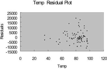
Many Factors Determine the Attendance at Major League

question 30

True/False

TABLE 15-9
Many factors determine the attendance at Major League Baseball games. These factors can include when the game is played, the weather, the opponent, whether or not the team is having a good season, and whether or not a marketing promotion is held. Data from 80 games of the Kansas City Royals for the following variables are collected.
ATTENDANCE = Paid attendance for the game
TEMP = High temperature for the day
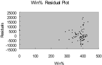
WIN% = Team's winning percentage at the time of the game
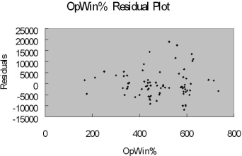
OPWIN% = Opponent team's winning percentage at the time of the game WEEKEND - 1 if game played on Friday, Saturday or Sunday; 0 otherwise PROMOTION - 1 = if a promotion was held; 0 = if no promotion was held
The regression results using attendance as the dependent variable and the remaining five variables as the independent variables are presented below.

$$\begin{array}{l}\text { Regression Statistics }\\\begin{array} { l r } \hline \text { Multiple R } & 0.5487 \\\text { R Square } & 0.3011 \\\text { Adjusted R Square } & 0.2538 \\\text { Standard Error } & 6442.4456 \\\text { Observations } & 80 \\\hline\end{array}\end{array}$$

$$\begin{array}{l}\text { ANOVA }\\\begin{array} { l c c c c c } \hline & \mathrm { df } & \text { SS } & \text { MS } & \text { F } & \text { Significance } \mathrm { F } \\\hline \text { Regression } & 5 & 1322911703.0671 & 264582340.6134 & 6.3747 & 0.0001 \\\text { Residual } & 74 & 3071377751.1204 & 41505104.7449 & & \\\text { Total } & 79 & 4394289454.1875 & & & \\\hline\end{array}\end{array}$$

$\begin{array}{lrrrr}\hline&\text{Coefficients}&\text{ Standard Error}&\text{ t Stat}&\text{p-value}\\\hline\text{Intercept}&-3862.4808&6180.9452&-0.6249&0.5340\\\text { Temp } & 51.7031 & 62.9439 & 0.8214 & 0.4140 \\\text { Win\% } & 21.1085 & 16.2338 & 1.3003 & 0.1975 \\\text { OpWin\% } & 11.3453 & 6.4617 & 1.7558 & 0.0833 \\\text { Weekend } & 367.5377 & 2786.2639 & 0.1319 & 0.8954 \\\text { Promotion } & 6927.8820 & 2784.3442 & 2.4882 & 0.0151 \\\hline\end{array}$










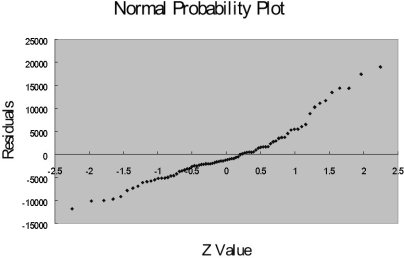
The coefficient of multiple determination ( R ² j) of each of the 5 predictors with all the other remaining predictors are, respectively, 0.2675, 0.3101, 0.1038, 0.7325, and 0.7308.

-Referring to Table 15-9, there is enough evidence to conclude that PROMOTION makes a significant contribution to the regression model in the presence of the other independent variables at a 5% level of significance.

---

Definitions:

Net Loss

The amount by which a company's expenses exceed its revenues, indicating that the business has spent more than it has earned in a specific period.

Total Cost Method

An accounting method that includes all costs related to the production of goods when calculating inventory cost.

Nonproduction Costs

Expenses not directly associated with the manufacturing or production of goods, such as selling, administrative, and other overhead costs.

Production Costs

Expenses directly associated with the creation of goods or services, including raw materials, direct labor, and manufacturing overhead.