SCENARIO 17-2 One of the most common questions of prospective house buyers pertains to the cost of heating in dollars (Y) . To provide its customers with information on that matter, a large real estate firm used the following 4 variables to predict heating costs: the daily minimum outside temperature in degrees of Fahrenheit (X1) , the amount of insulation in inches (X2) , the number of windows in the house (X3) , and the age of the furnace in years (X4) . Given below are the EXCEL outputs of two regression models.
Model 1
Regression Statistics R Square Adjusted R Square Observations 0.80800.756820 ANOVA
Regression Residual Total df41519 SS 169503.424140262.3259209765.75MS42375.862684.155F15.7874 Significance F0.0000
Intereept X1 (Temperature) X2 (Insulation) X3 (Windows) X4 (Furnace Age) Coefficients 421.4277−4.5098−14.90290.21516.3780 Standard Error 77.86140.81295.05084.86754.1026 t Stat 5.4125−5.5476−2.95050.04421.5546 P-value 0.00000.00000.00990.96530.1408 Lower 90.0% 284.9327−5.9349−23.7573−8.3181−0.8140 Upper 90.0% 557.9227−3.0847−6.04858.748413.5702
Model 2
Regression Statistics R Square Adjusted R Square Observations 0.77680.750620
ANOVA
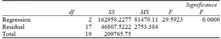
Intercept X1 (Temperature) X2 (Insulation) Coefficients 489.3227−5.1103−14.7195 Standard Error 43.98260.69514.8864t Stat 11.1253−7.3515−3.0123 P-value 0.00000.00000.0078 Lower 95% 396.5273−6.5769−25.0290 Upper 95% 582.1180−3.6437−4.4099
-Referring to Scenario 17-2, what are the degrees of freedom of the partial F test for H0:β3=β4=0 vs. H1: At least one βj=0,j=3,4 ?
McKinley's Victory
Refers to the election win of William McKinley in the 1896 United States presidential election, which was significant for its emphasis on economic issues.
Pullman Strike
A nationwide railroad strike in the United States in 1894, triggered by wage reductions at the Pullman Company and leading to a significant labor conflict.
National Rail Service
A network of trains operated by one or more companies, providing nationwide train transportation in a specific country.
Eugene V. Debs
An American socialist, political activist, and trade unionist, known for his role in founding the Industrial Workers of the World and for running unsuccessfully for U.S. president five times as a candidate of the Socialist Party.