SCENARIO 17-10 Given Below Are Results from the Regression Analysis $1 =$

question 162

True/False

SCENARIO 17-10 Given below are results from the regression analysis where the dependent variable is the number of weeks a worker is unemployed due to a layoff (Unemploy) and the independent variables are the age of the worker (Age), the number of years of education received (Edu), the number of years at the previous job (Job Yr), a dummy variable for marital status (Married: $1 =$ married, $0 =$ otherwise), a dummy variable for head of household (Head: $1 =$ yes, $0 =$ no) and a dummy variable for management position (Manager: $1 =$ yes, $0 =$ no). We shall call this Model 1. The coefficient of partial determination ( $R _ { \mathrm { y } } ^ { 2 }$ (All raiables excopt $j$ ) ) of each of the 6 predictors are, respectively, $0.2807$ , $0.0386,0.0317,0.0141,0.0958$ , and $0.1201$ .

$\begin{array}{lr}\hline{\text { Regression Statistics }} \\\hline \text { Multiple R } & 0.7035 \\\text { R Square } & 0.4949 \\\text { Adjusted R } & 0.4030 \\\text { Square } & \\\text { Standard } & 18.4861 \\\text { Error } & \\\text { Observations } & 40 \\\hline\end{array}$
$\text { ANOVA }$



$$\begin{array}{l}\begin{array} { l r r r r r r } \hline & \text { Coefficients } & \text { Standard Error } & { t \text { Stat } } & \text { P-value } & \text { Lower 95\% } & \text { Upper 95\% } \\\hline \text { Intercept } & 32.6595 & 23.18302 & 1.4088 & 0.1683 & - 14.5067 & 79.8257 \\\text { Age } & 1.2915 & 0.3599 & 3.5883 & 0.0011 & 0.5592 & 2.0238 \\\text { Edu } & - 1.3537 & 1.1766 & - 1.1504 & 0.2582 & - 3.7476 & 1.0402 \\\text { Job Yr } & 0.6171 & 0.5940 & 1.0389 & 0.3064 & - 0.5914 & 1.8257 \\\text { Married } & - 5.2189 & 7.6068 & - 0.6861 & 0.4974 & - 20.6950 & 10.2571 \\\text { Head } & - 14.2978 & 7.6479 & - 1.8695 & 0.0704 & - 29.8575 & 1.2618 \\\text { Manager } & - 24.8203 & 11.6932 & - 2.1226 & 0.0414 & - 48.6102 & - 1.0303 \\\hline\end{array}\end{array}$$
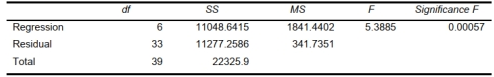
-Referring to Scenario 17-10 Model 1 Model 1, the null hypothesis $$H _ { 0 } : \beta _ { 1 } = \beta _ { 2 } = \beta _ { 3 } = \beta _ { 4 } = \beta _ { 5 } = \beta _ { 6 } = 0$$ implies that the number of weeks a worker is
unemployed due to a layoff is not affected by any of the explanatory variables.

---

Definitions:

Labor

Pertains to the utilization of human labor, encompassing both physical and intellectual efforts, in the creation of products and services.

Marginal Rate

Often referred to in the context of taxes or production, indicating the rate of increase or the additional cost or benefit of producing one more unit of a good.

Technical Substitution

The process of replacing one input or factor of production with another to maintain the same level of output.

Marginal Product

The additional output that results from adding one more unit of a specific input, keeping all other inputs constant.