SCENARIO 17-10 Given Below Are Results from the Regression Analysis $1 =$

question 300

True/False

SCENARIO 17-10 Given below are results from the regression analysis where the dependent variable is the number of weeks a worker is unemployed due to a layoff (Unemploy) and the independent variables are the age of the worker (Age), the number of years of education received (Edu), the number of years at the previous job (Job Yr), a dummy variable for marital status (Married: $1 =$ married, $0 =$ otherwise), a dummy variable for head of household (Head: $1 =$ yes, $0 =$ no) and a dummy variable for management position (Manager: $1 =$ yes, $0 =$ no). We shall call this Model 1. The coefficient of partial determination ( $R _ { \mathrm { y } } ^ { 2 }$ (All raiables excopt $j$ ) ) of each of the 6 predictors are, respectively, $0.2807$ , $0.0386,0.0317,0.0141,0.0958$ , and $0.1201$ .

$\begin{array}{lr}\hline{\text { Regression Statistics }} \\\hline \text { Multiple R } & 0.7035 \\\text { R Square } & 0.4949 \\\text { Adjusted R } & 0.4030 \\\text { Square } & \\\text { Standard } & 18.4861 \\\text { Error } & \\\text { Observations } & 40 \\\hline\end{array}$
$\text { ANOVA }$



$$\begin{array}{l}\begin{array} { l r r r r r r } \hline & \text { Coefficients } & \text { Standard Error } & { t \text { Stat } } & \text { P-value } & \text { Lower 95\% } & \text { Upper 95\% } \\\hline \text { Intercept } & 32.6595 & 23.18302 & 1.4088 & 0.1683 & - 14.5067 & 79.8257 \\\text { Age } & 1.2915 & 0.3599 & 3.5883 & 0.0011 & 0.5592 & 2.0238 \\\text { Edu } & - 1.3537 & 1.1766 & - 1.1504 & 0.2582 & - 3.7476 & 1.0402 \\\text { Job Yr } & 0.6171 & 0.5940 & 1.0389 & 0.3064 & - 0.5914 & 1.8257 \\\text { Married } & - 5.2189 & 7.6068 & - 0.6861 & 0.4974 & - 20.6950 & 10.2571 \\\text { Head } & - 14.2978 & 7.6479 & - 1.8695 & 0.0704 & - 29.8575 & 1.2618 \\\text { Manager } & - 24.8203 & 11.6932 & - 2.1226 & 0.0414 & - 48.6102 & - 1.0303 \\\hline\end{array}\end{array}$$
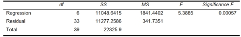
-Referring to Scenario 17-10 Model 1, the null hypothesis $$H _ { 0 } : \beta _ { 1 } = \beta _ { 2 } = \beta _ { 3 } = \beta _ { 4 } = \beta _ { 5 } = \beta _ { 6 } = 0$$ implies that the number of weeks a worker is
unemployed due to a layoff is not affected by some of the explanatory variables.

---

Definitions:

Financial Crises

Periods of significant financial instability and distress in an economy, characterized by rapid devaluation of assets, bank failures, and loss of investor confidence.

Labor Shortages

A situation where there are insufficient qualified candidates to fill the available jobs in the market, often leading to operational challenges for businesses.

Economic Factors

Elements that influence economic performance and decision-making, including inflation, interest rates, economic growth, and government policies.

Inputs and Outputs

The terms refer to the information or materials that are put into a system (inputs) and the results or products that come out of the system (outputs).