SCENARIO 17-10 Given below are results from the regression analysis where the dependent variable is the number of weeks a worker is unemployed due to a layoff (Unemploy) and the independent variables are the age of the worker (Age), the number of years of education received (Edu), the number of years at the previous job (Job Yr), a dummy variable for marital status (Married: 1= married, 0= otherwise), a dummy variable for head of household (Head: 1= yes, 0= no) and a dummy variable for management position (Manager: 1= yes, 0= no). We shall call this Model 1. The coefficient of partial determination ( Ry2 (All raiables excopt j ) ) of each of the 6 predictors are, respectively, 0.2807 , 0.0386,0.0317,0.0141,0.0958 , and 0.1201 .
Regression Statistics Multiple R R Square Adjusted R Square Standard Error Observations 0.70350.49490.403018.486140
ANOVA
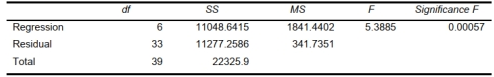
Intercept Age Edu Job Yr Married Head Manager Coefficients 32.65951.2915−1.35370.6171−5.2189−14.2978−24.8203 Standard Error 23.183020.35991.17660.59407.60687.647911.6932t Stat 1.40883.5883−1.15041.0389−0.6861−1.8695−2.1226 P-value 0.16830.00110.25820.30640.49740.07040.0414 Lower 95% −14.50670.5592−3.7476−0.5914−20.6950−29.8575−48.6102 Upper 95% 79.82572.02381.04021.825710.25711.2618−1.0303
-Referring to Scenario 17-10 Model 1, the alternative hypothesis H1 : At least one of βj=0 for j = 1, 2, 3, 4, 5, 6 implies that the number of weeks a worker is unemployed due to a layoff is
related to all of the explanatory variables.
Definitions:
Supply Chain Decision-Making
The process of strategizing, planning, and executing actions across the supply chain to optimize operations and performance.
Competitive Strategy
A method businesses use to achieve a competitive advantage by planning how to outperform their rivals.
Cycle Inventory
The average amount of inventory used to satisfy demand between orders, part of the total inventory that cycles through the supply chain.
Supplier Shipments
Deliveries of goods or materials from suppliers to manufacturers, retailers, or other entities in the supply chain.