14-22 Introduction to Multiple Regression One of the most common questions of prospective house buyers pertains to the cost of heating in dollars . To provide its customers with information on that matter, a large real estate firm used the following 2 variables to predict heating costs: the daily minimum outside temperature in degrees of Fahrenheit and the amount of insulation in inches . Given below is EXCEL output of the regression model.
ANOVA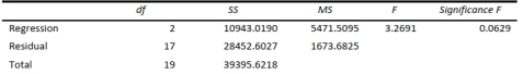
Also and
-Referring to Scenario 14-6, the partial F test for : Variable does not significantly improve the model after variable has been included : Variable significantly improves the model after variable has been included has and degrees of freedom.
Definitions:
Labour and Overhead
Combined costs associated with the workforce (labour) and indirect expenses (overhead) necessary for production but not directly tied to specific units of product.
Process Costing System
An accounting method used where production is continuous, assigning costs to units of product based on the processes they undergo.
Weighted-Average Method
An inventory costing method that calculates the cost of ending inventory and cost of goods sold based on the average cost of all similar items in the inventory.
Process Costing System
An accounting method used where goods are produced in a continuous process, costs are averaged over the units produced to determine per unit cost.
Q33: Referring to Scenario 14-12, if one is
Q79: Referring to Scenario 16-13, if a five-month
Q130: Referring to Scenario 16-3, if this series
Q133: The coefficient of determination represents the ratio
Q191: If a categorical independent variable contains 4
Q201: Referring to Scenario 13-11, what arethe lower
Q223: Referring to Scenario 14-7, the department
Q235: Referring to Scenario 14-2, an employee who
Q266: A regression had the following results: SST
Q357: Referring to Scenario 14-15, you can