SCENARIO 14-8 a Financial Analyst Wanted to Examine the Relationship $\$ 1,000$

question 31

Short Answer

SCENARIO 14-8 A financial analyst wanted to examine the relationship between salary (in $\$ 1,000$ ) and 2 variables: age $\left(X_{1}=\mathrm{Age}\right)$ and experience in the field $\left(X_{2}=\right.$ Exper). He took a sample of 20 employees and obtained the following Microsoft Excel output:

$\begin{array}{lr}\hline {\text { Regression Statistics }} \\\hline \text { Multiple R } & 0.8535 \\\text { R Square } & 0.7284 \\\text { Adjusted R Square } & 0.6964 \\\text { Standard Error } & 10.5630 \\\text { Observations } & 20 \\\hline\end{array}$

$\text { ANOVA }$


$\begin{array}{lrrrrrr} & \text { Coefficients } & \text { Standard Error } & {\text { t Stat }} & \text { P-value } & \text { Lower 95\% } &{\text { O5\% }} \\\hline \text { Intercept } & 1.5740 & 9.2723 & 0.1698 & 0.8672 & -17.9888 & 21.1368 \\\text { Age } & 1.3045 & 0.1956 & 6.6678 & 0.0000 & 0.8917 & 1.7173 \\\text { Exper } & -0.1478 & 0.1944 & -0.7604 & 0.4574 & -0.5580 & 0.2624 \\\hline\end{array}$
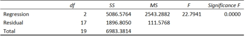
Also the sum of squares due to the regression for the model that includes only Age is 5022.0654 while the
sum of squares due to the regression for the model that includes only Exper is 125.9848.
-Referring to Scenario 14-8, the coefficient of partial determination $r _ { Y 1 \cdot 2 } ^ { 2 }$ ⋅ is ____.

---

Definitions:

Farm

An area of land and its buildings, used for growing crops and raising animals.

Production Level

Refers to the amount of goods or services produced by a company or industry over a specific time period.

Variable Costs

Expenses that fluctuate in direct proportion to production levels or output, including labor and materials.

Short-run Supply Curve

A graphical representation of the quantity of goods a firm is willing and able to supply to the market at different prices, over a short period where at least one input is fixed.