You Learned in Intermediate Macroeconomics That Certain Macroeconomic Growth Models

question 20

Essay

You learned in intermediate macroeconomics that certain macroeconomic growth models predict conditional convergence or a catch up effect in per capita GDP between the countries of the world.That is,countries which are further behind initially in per-capita GDP will grow faster than the leader.You gather data from the Penn World Tables to test this theory.
(a)By limiting your sample to 24 OECD countries,you hope to have a more homogeneous set of countries in your sample,i.e. ,countries that are not too different with respect to their institutions.To simplify matters,you decide to only test for unconditional convergence.In that case,the laggards catch up even without taking into account differences in some of the driving variables.Your scatter plot and regression for the time period 1975-1989 are as follows: 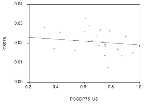= 0.024 - 0.005 PCGDP75_US;R2= 0.025,SER = 0.006
(0.06)(0.008)
where is the average annual growth rate of per capita GDP from 1975-1989,and PCGDP75_US is per capita GDP relative to the United States in 1975.Numbers in parenthesis are heteroskedasticity-robust standard errors.
Interpret the results.Is there indication of unconditional convergence? What critical value did you use?
(b)Although you are quite discouraged by the result,you think that it might be due to the specific time period used.During this period,there were two OPEC oil price shocks with varying degrees of exposure for the OECD countries.You therefore repeat the exercise for the period 1960-1974,with the following results: 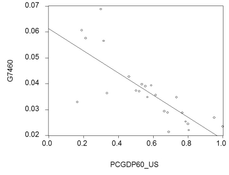= 0.061 - 0.043 PCGDP60_US;R2= 0.613,SER = 0.008
(0.004)(0.007)
where is the average annual growth rate of per capita GDP from 1960-1974,and PCGDP60_US is per capita GDP relative to the United States in 1960.
Compare this regression to the previous one.
(c)You decide to run one more regression in differences.The dependent variable is now the change in the growth rate of per capita GDP from 1960-1974 to 1975-1989 (diffg)and the regressor the difference in the initial conditions (diffinit).This produces the following graph and regression: = -0.006 - 0.096 × diffinit;R2 = 0.468;SER = 0.009
(0.03)(0.021)
Interpret these results.Explain what has happened to unobservable omitted variables that are constant over time.Suggest what some of these variables might be.
(d)Given that there are only two time periods,what other methods could you have employed to generate the identical results? Why do you think that the slope coefficient in this regression is significant given the results over the sub-periods?

Compute unrealized intercompany profits and their eliminations in consolidated financial statements.

Calculate depreciation and its adjustments in intercompany asset transactions.

Calculate and adjust for intercompany dividends received.

Understand the impact of intercompany transactions on consolidated net income and retained earnings.

---

Definitions:

Process Layouts

An arrangement of resources in a production facility where similar activities or functions are grouped together, based on the type of process they are involved in.

Relative Positioning

The strategic process of establishing a brand or product's identity by comparing it to and differentiating it from competitors in the marketplace.

Fixed-position Layouts

A type of industrial layout where the product remains stationary, and equipment, labor, and components are moved as needed to the product's location for assembly or construction.

Off-site

Off-site refers to activities or processes that are conducted away from the primary location or site, often implying external premises.