SCENARIO 17-2 One of the most common questions of prospective house buyers pertains to the cost of heating in dollars (Y) . To provide its customers with information on that matter, a large real estate firm used the following 4 variables to predict heating costs: the daily minimum outside temperature in degrees of Fahrenheit (X1) , the amount of insulation in inches (X2) , the number of windows in the house (X3) , and the age of the furnace in years (X4) . Given below are the EXCEL outputs of two regression models.
Model 1
Regression Statistics R Square Adjusted R Square Observations 0.80800.756820 ANOVA
Regression Residual Total df41519 SS 169503.424140262.3259209765.75MS42375.862684.155F15.7874 Significance F0.0000
Intereept X1 (Temperature) X2 (Insulation) X3 (Windows) X4 (Furnace Age) Coefficients 421.4277−4.5098−14.90290.21516.3780 Standard Error 77.86140.81295.05084.86754.1026 t Stat 5.4125−5.5476−2.95050.04421.5546 P-value 0.00000.00000.00990.96530.1408 Lower 90.0% 284.9327−5.9349−23.7573−8.3181−0.8140 Upper 90.0% 557.9227−3.0847−6.04858.748413.5702
Model 2
Regression Statistics R Square Adjusted R Square Observations 0.77680.750620
ANOVA
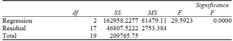
Intercept X1 (Temperature) X2 (Insulation) Coefficients 489.3227−5.1103−14.7195 Standard Error 43.98260.69514.8864t Stat 11.1253−7.3515−3.0123 P-value 0.00000.00000.0078 Lower 95% 396.5273−6.5769−25.0290 Upper 95% 582.1180−3.6437−4.4099
-Referring to Scenario 17-2, what are the degrees of freedom of the partial F test for H0:β3=β4=0 vs. H1: At least one βj=0,j=3,4 ?
Activity Rates
Rates used in activity-based costing to assign costs to products or services based on the amount of an activity they consume.
Activity-Based Costing
A method of costing that identifies individual activities as the fundamental cost objects and uses the costs of these activities to compute the costs of various products or services.
Direct Labor-Hours
The total hours worked by employees directly involved in the production process, often used as a basis for allocating overhead costs.
Product J3
Product J3 could refer to a specific model or item within a company's lineup, identified by the code "J3."